The Weather Station uses the Weatherduino hardware and software to collect and process the data from the varous sensors, and a Raspberry Pi computer running a program called CumulusMX (CMX) to interrogate the receiver and interact with various websites. CumulusMX is the latest incarnation of a program originally developed by Steve Loft (Sandaysoft) and now maintained by Mark Crossley. Earlier versions of Cumulus are still available (although mostly unsupported), but CumulusMX has several advantages. For example it runs on different operating systems and it has enhanced data processing routines that are triggered either at the end of each day or by specific events.

Station settings

This is where you enter the details of your weather station, including the sensors used, the units of measurement and the location of the site. I had to change the default serial port to /dev/ttyACM0 with my Raspberry Pi. I set CumulusMX to log the data from the Weatherduino every 5 minutes.

Internet settings

In this section you enter the information needed to send data via FTP to your website, including how frequently you want to upload data (I have mine set at 30 minutes).

Extra web files

Cumulus is able to upload files to a website at different intervals. First, files can be uploaded at the ‘real-time’ interval which is typically set to 15-30 seconds, which can be useful for rapidly changing phenomena or when a display such as a simulated analogue gauge is needed. Second, data can be uploaded at the normal sample interval, which is every 30 minutes in my case. Finally, data can be uploaded at the end of the day, as part of the routine ‘clean up’ of data files that Cumulus undertakes. Even more powerful is the option to process any of these files, replacing ‘web-tags’ with actual data drawn from the weather station. This provides a flexible and effective way to generate bespoke web pages at different time intervals.

Calibration settings

Self-explanatory. This section allows you to enter offsets and multipliers as well as apply some simple data cleaning & validation.

NOAA settings

Tweak the content of standardised NOAA monthly and yearly reports.

MySQL settings

Allows you to create daily or monthly tables of data. I have my station set up to generate a monthly table in which data are collected every 5 minutes and uploaded to a MySQL database on my website every 30 minutes. These data can then be used to generate graphs and tables of historic data, as well as providing a back-up of the data collected. I have also configured CumulusMX to regularly update a ‘dayfile’ in which each row is a summary of that day’s most important data. This file is uploaded to my website as part of the ‘end of day’ processing. An example of a chart created from this file is shown below. The chart was produced from the dayfile using ‘R’.

Alarms

Self-explanatory. Sets audible alarms based on extreme values.

FTP Now!

Manually initiate the FTP process.

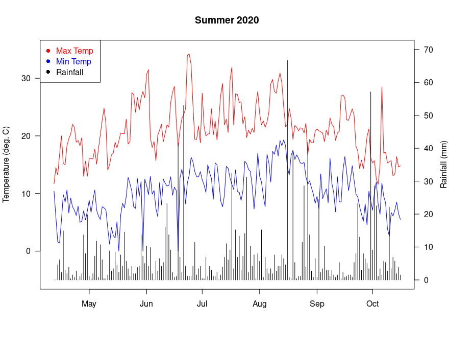
# R Program to plot summary data from dayfile1.csv
# Plots Max & Min temp as well as rainfall
# ** Line continuation symbols not shown **
#
# Read in data in csv format. First row contains variable names.
dayfile <- read.csv("~/Documents/CMX/SummaryReports/dayfile1.csv", header=TRUE)

# Convert LogDate to simple date format
dayfile$Date <- as.Date(dayfile$LogDate,format="%Y-%m-%d")

## add extra space to right margin of plot within frame
par(mar=c(6, 4, 4, 6) + 0.1)

# Plot daily minimum temperature
plot(dayfile$Date, dayfile$"MinTemp", xlab="", ylab="", ylim=c(-5,35), axes=FALSE, type="l", main="Summer 2020", col="blue")
axis(2, ylim=c(-5,35), col="black", las=1)
mtext("Temperature (deg. C)", side=2, line=3)
box()

# Plot daily maximum temperature
## Allow a second plot on the same graph
par(new=TRUE)
plot(dayfile$Date, dayfile$"MaxTemp", xlab="", ylab="", ylim=c(-5,35), axes=FALSE, type="l", col="red")

# Plot rainfall as type 'h' (histogram/lines)
par(new=TRUE)
## Plot the third plot and put axis scale on right
plot(dayfile$Date, dayfile$"TotRainFall", xlab="", ylab="", ylim=c(0, 70), axes=FALSE, type="h", col="black")

## a little farther out (line=4) to make room for labels
mtext("Rainfall (mm)",side=4,col="black",line=2.5) 
axis(4, ylim=c(0,60), col="black",col.axis="black",las=1)

## Add Legend
legend("topleft",legend=c("Max Temp","Min Temp","Rainfall"),text.col=c("red","blue","black"),pch=c(16,16,16),col=c("red","blue","black"))

## Draw the time axis
axis.Date(side=1, dayfile$Date, col="black", line=0)

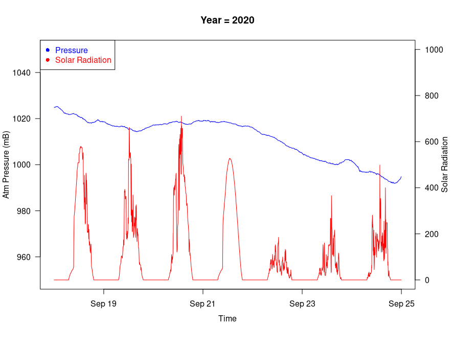
# Plots Pressure and Solar Radiation over several days, extracted from Monthly data file
#
# Line continuation symbols not shown
#
# Read in monthly data file
Oct20data <- read.csv("~/Documents/CMX/SummaryReports/Oct20data.csv", header=TRUE)

# Create meaningful time variable
Oct20data$UnixTime <- as.POSIXct(Oct20data$LogDateTime, format= "%Y-%m-%d %H:%M:%S")

## add extra space to right margin of plot within frame
par(mar=c(6, 4, 4, 6) + 0.1)

#Create subset to plot
newdata <- subset(Oct20data, UnixTime >= "2020-09-18 00:00:00" & UnixTime < "2020-09-25 00:00:00" , select = c(UnixTime,Pressure,SolarRad))

# Plot the subset
plot(newdata$UnixTime, newdata$Pressure, ylim=c(950,1050), axes=FALSE, type="l", main="Year = 2020", xlab="", ylab="", col="blue")
axis(2, ylim=c(950,1050), col="black", las=1)
mtext("Atm Pressure (mB)", side=2, line=3)
box()

## Allow a second plot on the same graph
par(new=TRUE)
## Plot the second plot and put axis scale on right
plot(newdata$UnixTime, newdata$SolarRad, xlab="", ylab="", ylim=c(0,1000),axes=FALSE, type="l", col="red")
## a little farther out (line=4) to make room for labels
mtext("Solar Radiation",side=4,col="black",line=2.5) 
axis(4, ylim=c(0,1000), col="black",col.axis="black",las=1)

## Add Legend
legend("topleft",legend=c("Pressure","Solar Radiation"),text.col=c("blue","red"),pch=c(16,16),col=c("blue","red"))

## Draw the time axis
axis.POSIXct(side=1, newdata$UnixTime, col="black", line=0)
mtext("Time",side=1,col="black",line=2.5)